Project 9 - 유저 군집 분석

August 25, 2024 21 분 소요

클러스터링, 군집화

데이터가 주어졌을 때, 여러 개의 그룹으로 나누는 것
유사한 특성을 가진 그룹을 발견해내는 일

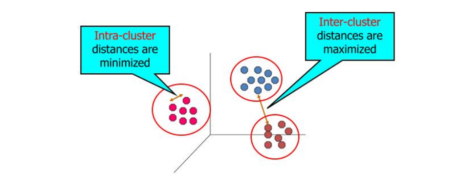
내부 멤버들 간의 사이(Intra-clust)는 가깝고, 그룬 간 사이(Inter-cluster)는 멀게 그룹을 만드는 것
그룹에 대한 정답이 있으면 분류 문제이지만 클러스터링은 비지도 학습으로 어느 그룹에 있는지 정답은 없다.

언제 사용할까?

유사한 뉴스 그룹 : 문서 군집화

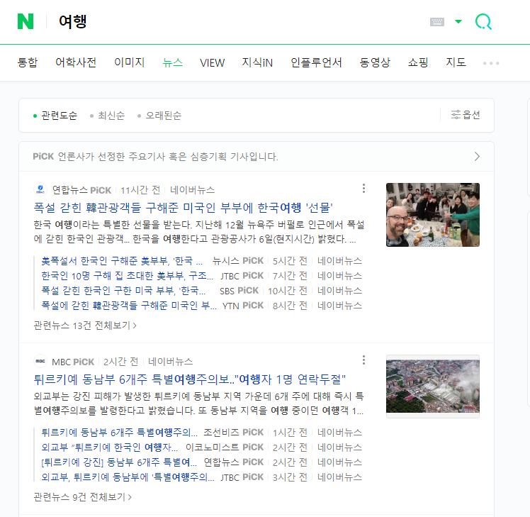
가까운 위치 좌표끼리 묶기

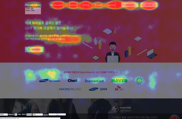
유사한 유저군 나누기 : 마켓 세분화

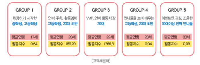
시장을 적절한 수로 나누고, 각 시장, 타겟 별로 효과적인 정책을 찾아낸다.

종류

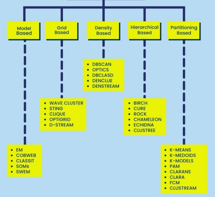
Partition-based Clustering

미리 군집(그룹)의 수를 정해두고 클러스터링하는 방식
대표적인 알고리즘
- K-means
- K-Medoids

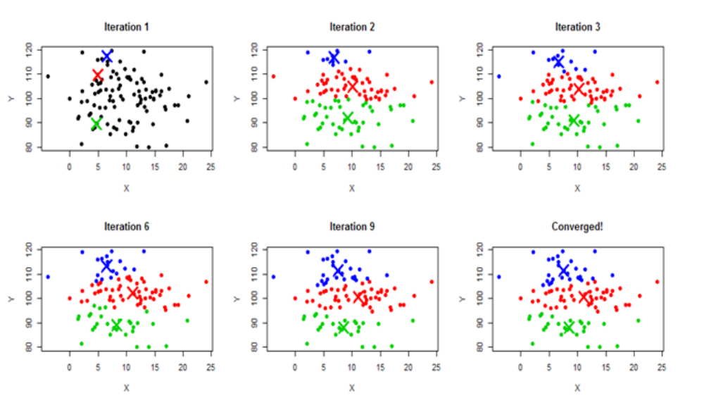
### K-means Clustering

사용자가 미리 군집수(k) 정의
처음에는 랜덤으로 k개의 중심점(Centroid)를 정함 - 각 군집은 하나의 중심(Centroid)를 가지고 있다.
데이터 point를 돌면서 가까운 중심점이 있는 그룹에 각 데이터를 할당 - 이 때 각 개체 간 거리는 Euclidean distance 사용
모두 그룹을 할당했다면, 각 그룹마다 새 중심점(Centroid) - 클러스터 내 평균점을 새로 구함
3-4 단계를 반복하다가 더 이상 그룹 이동이 일어나지 않으면 멈춤

Hierarchical based Clustering

여러개의 군집 중에서 가장 유사도가 높은 혹은 거리가 가까운 군집 두 개를 선택하여 하나로 합치면서 군집 개수를 줄여가는 방법으로 agglomerative clustering(합체 군집)라고도 한다.
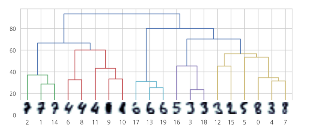
가까운 데이터를 서로 묶기 위해서는 먼저 각 군집 간 거리를 계산해야 한다.

Centroid Distance

각 군집의 중심점 사이의 거리를 계산하는 방법
계층 클러스터링이 아니더라도 사용할 수 있는 방법

Median Distance

Hierarchical based Clustering에서 사용할 수 있는 방법
군집 u가 군집 s와 군집 t의 결합으로 생성된 군집이라면, 중심점을 새로 계산하지 않고, 기존 s와 t의 중심점의 평균을 사용한다 -> 더 빠른 계산 가능

Density based Clustering

데이터가 밀집한 정도, 밀도를 이용한 클러스터링 방법

DBSCAN clustering

군집의 개수를 사용자가 지정할 필요가 없다.
초기 데이터로부터 근접한 데이터를 찾아나가는 방법으로 군집을 확장
필요한 파라미터는 2가지로 ‘근접하다’를 정의
- 최소거리 a (다른 점들을 이웃으로 묶기 위함)
- 최소 데이터 개수 b (밀집 지역으로 정의하기 위함)
최소거리 a안에 있는 데이터는 이웃이다.
최소거리 a안에 최소 데이터 개수 b 이상의 데이터가 있으면, 이 데이터를 core로 정의
core데이터는 하나의 클러스터를 형성하고, 그 core와 a 거리 내에 있는 점들은 같은 클러스터로 분류

K-means는 중심점을 기준으로 그룹을 형성하기 때문에, 원의 형태로 군집이 만들어짐
서로 이웃한 데이터들을 같은 클러스터에 포함시키기 때문에 불특정한 모양의 클러스터가 형성

정답이 없는 클러스터링, 어떻게 평가할까?

이미 정답이 있는 분류문제와 달리 성능 기준을 만들기 어렵다. 따라서 기준을 사용할 수 있지만, 그 중 클러스터에 대한 정답이 없는 경우 사용할 수 있는 기준을 알아보자

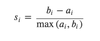
Silhouette Coefficient: 실루엣 계수

모든 데이터 쌍 (i, j)에 대한 거리나 dissimilarity를 구한다.
- a_i : i와 같은 군집에 속한 원소들의 평균 거리
- b_i : i와 다른 군집 중 가장 가까운 군집까지의 평균 거리

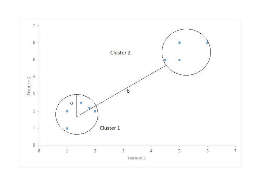
-> 만약 a 같은 군집 내 평균 거리가 더 가깝다면 양수, 다른 군집과의 거리가 가깝다면 음수가 나온다.

다양한 클러스터링 방법을 통해 유저 세그먼트를 나눠보자

라이브러리 불러오기

import pandas as pd
import numpy as np
import seaborn as sns
import matplotlib.pyplot as plt
from matplotlib import colors

👣 데이터 살펴보기

# 나의 구글 드라이브를 mount (colaboratory 노트북이 떠있는 위치에서 드라이브의 파일에 접근할 수 있게 만드는 것) 하는 명령어
from google.colab import drive
drive.mount('/content/drive')

# 판다스로 데이터 불러오기
# 아래에 customer_personality_analysis.csv 가 있는 경로로 이동합니다
# 경로 설정
DRIVE_PATH = "/content/drive/MyDrive/" # 내 드라이브의 경로이다
FILE_PATH_IN_MY_DRIVE = "zerobase/유저 데이터 분석/유저 군집 분석하기/data/customer_personality_analysis.csv" # 내 드라이브 내 파일이 있는 경로
PATH = DRIVE_PATH +  FILE_PATH_IN_MY_DRIVE

df = pd.read_csv(PATH , sep="\t") # csv 파일 읽어오기
df.head()

# ID,Year_Birth,Education
# ID\tYear\t

	ID	Year_Birth	Education	Marital_Status	Income	Kidhome	Teenhome	Dt_Customer	Recency	MntWines	...	NumWebVisitsMonth	Z_CostContact	Z_Revenue	Response
0	5524	1957	Graduation	Single	58138.0	0	0	04-09-2012	58	635	...	7	3	11	1
1	2174	1954	Graduation	Single	46344.0	1	1	08-03-2014	38	11	...	5	3	11	0
2	4141	1965	Graduation	Together	71613.0	0	0	21-08-2013	26	426	...	4	3	11	0
3	6182	1984	Graduation	Together	26646.0	1	0	10-02-2014	26	11	...	6	3	11	0
4	5324	1981	PhD	Married	58293.0	1	0	19-01-2014	94	173	...	5	3	11	0

print("데이터 전체의 행 수: ",len(df))
print("데이터 컬럼 수: ",len(df.columns))

=>

데이터 전체의 행 수:  2240
데이터 컬럼 수:  29

데이터 컬럼 종류

People (사람)

ID: Customer’s unique identifier
Year_Birth: Customer’s birth year
Education: Customer’s education level (교육 수준)
Marital_Status: Customer’s marital status (결혼 상태)
Income: Customer’s yearly household income
Kidhome: Number of children in customer’s household (어린 아이의 수)
Teenhome: Number of teenagers in customer’s household (10대 수)
Dt_Customer: Date of customer’s enrollment with the company (서비스 가입 날짜)
Recency: Number of days since customer’s last purchase (마지막으로 구매한 날로부터 얼마가 지났는지)
Complain: 1 if customer complained in the last 2 years, 0 otherwise

Products (상품)

MntWines: Amount spent on wine in last 2 years
MntFruits: Amount spent on fruits in last 2 years
MntMeatProducts: Amount spent on meat in last 2 years
MntFishProducts: Amount spent on fish in last 2 years
MntSweetProducts: Amount spent on sweets in last 2 years
MntGoldProds: Amount spent on gold in last 2 years

Promotion (프로모션)

NumDealsPurchases: Number of purchases made with a discount (할인 받아 구매한 수)
AcceptedCmp1: 1 if customer accepted the offer in the 1st campaign, 0 otherwise
AcceptedCmp2: 1 if customer accepted the offer in the 2nd campaign, 0 otherwise
AcceptedCmp3: 1 if customer accepted the offer in the 3rd campaign, 0 otherwise
AcceptedCmp4: 1 if customer accepted the offer in the 4th campaign, 0 otherwise
AcceptedCmp5: 1 if customer accepted the offer in the 5th campaign, 0 otherwise
Response: 1 if customer accepted the offer in the last campaign, 0 otherwise

Place (구매 장소)

NumWebPurchases: Number of purchases made through the company’s web site
NumCatalogPurchases: Number of purchases made using a catalogue
NumStorePurchases: Number of purchases made directly in stores
NumWebVisitsMonth: Number of visits to company’s web site in the last month

👣 데이터 정제하기: Cleaning

결측치 (Missing Values)와 이상치 (Outliers) 를 제거하자
데이터를 바로 사용할 수 있으면 좋겠지만, 바로 사용할 수 있는 경우가 많지 않다.
- 결측치가 있을 수 있고, 컴퓨터가 이해할 수 있는 형태 (숫자형)으로 바꿔주어야 하는 경우도 있다.
- Outlier 가 너무 크다면, 이상치로 인해 모델이 왜곡될 수 있다.

아래 데이터를 살펴보자

# .info() 함수는 데이터에 대한 전반적인 정보를 나타냅니다. 
# df를 구성하는 행과 열의 크기, 컬럼명, 컬럼을 구성하는 값의 자료형 등을 출력해줍니다.
df.info()

=>

<class 'pandas.core.frame.DataFrame'>
RangeIndex: 2240 entries, 0 to 2239
Data columns (total 29 columns):
 #   Column               Non-Null Count  Dtype  
---  ------               --------------  -----  
 ID                   2240 non-null   int64  
 Year_Birth           2240 non-null   int64  
 Education            2240 non-null   object 
 Marital_Status       2240 non-null   object 
 Income               2216 non-null   float64
 Kidhome              2240 non-null   int64  
 Teenhome             2240 non-null   int64  
 Dt_Customer          2240 non-null   object 
 Recency              2240 non-null   int64  
 MntWines             2240 non-null   int64  
MntFruits            2240 non-null   int64  
MntMeatProducts      2240 non-null   int64  
MntFishProducts      2240 non-null   int64  
MntSweetProducts     2240 non-null   int64  
MntGoldProds         2240 non-null   int64  
NumDealsPurchases    2240 non-null   int64  
NumWebPurchases      2240 non-null   int64  
NumCatalogPurchases  2240 non-null   int64  
NumStorePurchases    2240 non-null   int64  
NumWebVisitsMonth    2240 non-null   int64  
AcceptedCmp3         2240 non-null   int64  
AcceptedCmp4         2240 non-null   int64  
AcceptedCmp5         2240 non-null   int64  
AcceptedCmp1         2240 non-null   int64  
AcceptedCmp2         2240 non-null   int64  
Complain             2240 non-null   int64  
Z_CostContact        2240 non-null   int64  
Z_Revenue            2240 non-null   int64  
Response             2240 non-null   int64  
dtypes: float64(1), int64(25), object(3)
memory usage: 507.6+ KB

4 Income : non-null인 row의 수는 2216 개 - 비어있는 값이 24개 정도 있다.
7 Dt_Customer : 날짜형이지만 날짜가 아닌 String(object) 로 표시되어 있다.

결측치 제거하기

결측치를 제거하는 방법은 크게 3가지이다.
- 결측치의 비중이 작다면 제거한다.
- 결측치를 빈도가 가장 높은 값이나 평균으로 채운다.
- 결측치를 예측하는 모델을 만들어 예측값으로 채운다.
해당 데이터에서는 24개로 결측치가 많지 않기 때문에 제거한다.

# missing value 가 있는 row 를 제거한다.
# 결측치가 있는 경우 1. 평균치로 채우거나 2. 예측하거나 3. 데이터가 많지 않으면 제거한다.
df = df.dropna()
len(df)

=>

2216

날짜 데이터 정제하기

가입한지 얼마 되지 않은 고객과 가장 오래된 고객을 구해보자

# string으로 된 date 를 datetime 함수를 쓰기 위해 datetime 형태로 바꾼다.
# Dt_Customer: 가입한 날짜
df["Dt_Customer"] = pd.to_datetime(df["Dt_Customer"])

for i in df["Dt_Customer"][:5]:
  print(i.date())
  
=>

2012-04-09
2014-08-03
2013-08-21
2014-10-02
2014-01-19

dates = []
for i in df["Dt_Customer"]:
    i = i.date()
    dates.append(i)  
    
print(dates)
print(max(dates))
print(min(dates))

=>

[datetime.date(2012, 4, 9), datetime.date(2014, 8, 3), datetime.date(2013, 8, 21), ... , datetime.date(2014, 1, 25), datetime.date(2014, 1, 24), datetime.date(2012, 10, 15)]
2014-12-06
2012-01-08

날짜를 숫자로! 가입 날짜(date)를 가입한 후 지난 일수(int)로 바꿔준다.

days = [] # 데이터를 담을 수 있는 빈 list
recent_date = max(dates) # 2014-12-06, 
# 가장 최근 가입일 (해당 날짜를 기준으로 기존 날짜의 값을 빼준다.)
for date in dates:
    day_difference = recent_date - date
    days.append(day_difference)
df["Customer_For"] = days


df["Customer_For"].head()

=>

0   971 days
1   125 days
2   472 days
3    65 days
4   321 days
Name: Customer_For, dtype: timedelta64[ns]

# 날짜를 숫자로 type 을 변경해준다
df["Customer_For"] = pd.to_numeric(df["Customer_For"], errors="coerce")

# errors: error는 총 3개의 옵션이 존재합니다.
# errors = 'ignore' -> 만약 숫자로 변경할 수 없는 데이터라면 숫자로 변경하지 않고 원본 데이터를 그대로 반환합니다.
# errors = 'coerce' -> 만약 숫자로 변경할 수 없는 데이터라면 기존 데이터를 지우고 NaN으로 설정하여 반환합니다.
# errors = 'raise' -> 만약 숫자로 변경할 수 없는 데이터라면 에러를 일으키며 코드를 중단합니다.

카테고리 데이터 정리하기

앞에서 본 데이터 중 카테고리 형태의 데이터는 Education 과 Marital_Status :)

df[['Education', 'Marital_Status']].head(10)

	Education	Marital_Status
0	Graduation	Single
1	Graduation	Single
2	Graduation	Together
3	Graduation	Together
4	PhD	Married
5	Master	Together
6	Graduation	Divorced
7	PhD	Married
8	PhD	Together
9	PhD	Together

df["Marital_Status"].value_counts()

=>

Married     864
Together    580
Single      480
Divorced    232
Widow        77
Alone         3
Absurd        2
YOLO          2
Name: Marital_Status, dtype: int64

df["Education"].value_counts()

=>

Graduation    1127
PhD            486
Master         370
2n Cycle       203
Basic           54
Name: Education, dtype: int64

# Marital_Status 정리하기, 파트너와 같이 사는지, 혼자사는지 여부
df["Living_With"]=(
    df["Marital_Status"]
    .replace(
      {"Married":"Partner", 
       "Together":"Partner", 
       "Absurd":"Alone", 
       "Widow":"Alone", 
       "YOLO":"Alone", 
       "Divorced":"Alone", 
       "Single":"Alone"
    })
)

# the number of children, Kidhome 과 Teenhome 을 분리하지 않고 합쳐준다.
df["Children"]=df["Kidhome"]+df["Teenhome"]

# 위의 데이터를 통해 가족 사이즈도 구할 수 있다.
df["Family_Size"] = (
    df["Living_With"].replace({"Alone": 1, "Partner":2})
    + df["Children"]
)

# 아이가 있는지, 없는지
df["Is_Parent"] = np.where(df.Children> 0, 1, 0)

# 교육 상태 정리하기
df["Education"]=df["Education"].replace({"Basic":"Undergraduate","2n Cycle":"Undergraduate", "Graduation":"Graduate", "Master":"Postgraduate", "PhD":"Postgraduate"})

# 생년 월일을 통해 나이를 구할 수 있다.
df["Age"] = 2021-df["Year_Birth"]

# 다양한 잡화 구매를 더해서 총 사용한 비용 Spent 를 구한다.
df["Spent"] = df["MntWines"]+ df["MntFruits"]+ df["MntMeatProducts"]+ df["MntFishProducts"]+ df["MntSweetProducts"]+ df["MntGoldProds"]

# 모두 동일한 값, 필요없는 컬럼
df.Z_CostContact.value_counts()
df.Z_Revenue.value_counts()

=>

11    2216
Name: Z_Revenue, dtype: int64

# 컬럼명 짧게 변경
df=df.rename(columns={"MntWines": "Wines","MntFruits":"Fruits","MntMeatProducts":"Meat","MntFishProducts":"Fish","MntSweetProducts":"Sweets","MntGoldProds":"Gold"})

# 중복되거나 필요없는 컬럼 제거
to_drop = ["Marital_Status", "Dt_Customer", "Z_CostContact", "Z_Revenue", "Year_Birth", "ID"]
df = df.drop(to_drop, axis=1)


df.head()

	Education	Income	Kidhome	Teenhome	Recency	Wines	Fruits	Meat	Fish	Sweets	...	Response	Customer_For	Living_With	Children	Family_Size	Is_Parent	Age	Spent
0	Graduate	58138.0	0	0	58	635	88	546	172	88	...	1	83894400000000000	Alone	0	1	0	64	1617
1	Graduate	46344.0	1	1	38	11	1	6	2	1	...	0	10800000000000000	Alone	2	3	1	67	27
2	Graduate	71613.0	0	0	26	426	49	127	111	21	...	0	40780800000000000	Partner	0	2	0	56	776
3	Graduate	26646.0	1	0	26	11	4	20	10	3	...	0	5616000000000000	Partner	1	3	1	37	53
4	Postgraduate	58293.0	1	0	94	173	43	118	46	27	...	0	27734400000000000	Partner	1	3	1	40	422

Outlier 제거하기 우리가 정리한 데이터를 다시 한 번 살펴보자

 df.describe()

	Income	Kidhome	Teenhome	Recency	Wines	Fruits	Meat	Fish	Sweets	Gold	...	AcceptedCmp1	AcceptedCmp2	Complain	Response	Customer_For	Children	Family_Size	Is_Parent	Age	Spent
count	2216.000000	2216.000000	2216.000000	2216.000000	2216.000000	2216.000000	2216.000000	2216.000000	2216.000000	2216.000000	...	2216.000000	2216.000000	2216.000000	2216.000000	2.216000e+03	2216.000000	2216.000000	2216.000000	2216.000000	2216.000000
mean	52247.251354	0.441787	0.505415	49.012635	305.091606	26.356047	166.995939	37.637635	27.028881	43.965253	...	0.064079	0.013538	0.009477	0.150271	4.423735e+16	0.947202	2.592509	0.714350	52.179603	607.075361
std	25173.076661	0.536896	0.544181	28.948352	337.327920	39.793917	224.283273	54.752082	41.072046	51.815414	...	0.244950	0.115588	0.096907	0.357417	2.008532e+16	0.749062	0.905722	0.451825	11.985554	602.900476
min	1730.000000	0.000000	0.000000	0.000000	0.000000	0.000000	0.000000	0.000000	0.000000	0.000000	...	0.000000	0.000000	0.000000	0.000000	0.000000e+00	0.000000	1.000000	0.000000	25.000000	5.000000
25%	35303.000000	0.000000	0.000000	24.000000	24.000000	2.000000	16.000000	3.000000	1.000000	9.000000	...	0.000000	0.000000	0.000000	0.000000	2.937600e+16	0.000000	2.000000	0.000000	44.000000	69.000000
50%	51381.500000	0.000000	0.000000	49.000000	174.500000	8.000000	68.000000	12.000000	8.000000	24.500000	...	0.000000	0.000000	0.000000	0.000000	4.432320e+16	1.000000	3.000000	1.000000	51.000000	396.500000
75%	68522.000000	1.000000	1.000000	74.000000	505.000000	33.000000	232.250000	50.000000	33.000000	56.000000	...	0.000000	0.000000	0.000000	0.000000	5.927040e+16	1.000000	3.000000	1.000000	62.000000	1048.000000
max	666666.000000	2.000000	2.000000	99.000000	1493.000000	199.000000	1725.000000	259.000000	262.000000	321.000000	...	1.000000	1.000000	1.000000	1.000000	9.184320e+16	3.000000	5.000000	1.000000	128.000000	2525.000000

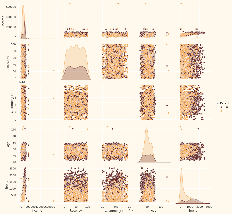
-> Income 과 Age 의 Max 를 보자. Outlier 가 숨어있는 것 같다!

# 색상 지정
sns.set(rc={"axes.facecolor":"#FFF9ED","figure.facecolor":"#FFF9ED"})
pallet = ["#682F2F", "#9E726F", "#D6B2B1", "#B9C0C9", "#9F8A78", "#F3AB60"]
cmap = colors.ListedColormap(["#682F2F", "#9E726F", "#D6B2B1", "#B9C0C9", "#9F8A78", "#F3AB60"])

# 아래의 정해진 컬럼들 사이의 상관관계를 그래프로 확인해 본다.
To_Plot = [ "Income", "Recency", "Customer_For", "Age", "Spent", "Is_Parent"]
print("Reletive Plot Of Some Selected Features: A Data Subset")
sns.pairplot(df[To_Plot], hue= "Is_Parent", palette=(["#682F2F","#F3AB60"]))

# Outlier (Age, Income) 삭제
df = df[(df["Age"]< 90)]
df = df[(df["Income"] < 600000)]
print("Outlier 제거 후 데이터 row 수:", len(df))


# box plot 이나 분포를 보고도 알 수 있음.

=>

Outlier 제거 후 데이터 row 수: 2212

💡 Correlation Coefficients

correlation (상관성)이란?
- 상관성은 두 변수간의 “선형적” 관계의 정도를 의미
- -1 ~ 1 사이를 가지며 1에 가까울 수록 양의 선형관계, -1에 가까울 수록 음의 선형관계가 강하다는 것을 의미

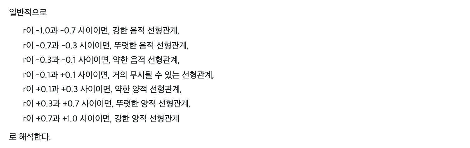
df.corr()

	Income	Kidhome	Teenhome	Recency	Wines	Fruits	Meat	Fish	Sweets	Gold	...	AcceptedCmp1	AcceptedCmp2	Complain	Response	Customer_For	Children	Family_Size	Is_Parent	Age	Spent
Income	1.000000	-0.514523	0.034565	0.007965	0.688209	0.507354	0.692279	0.520040	0.523599	0.388299	...	0.327524	0.104036	-0.027900	0.161387	-0.027892	-0.343529	-0.286638	-0.403132	0.199977	0.792740
Kidhome	-0.514523	1.000000	-0.039066	0.010623	-0.497203	-0.373258	-0.439031	-0.388643	-0.377843	-0.354922	...	-0.174261	-0.081911	0.037067	-0.077901	-0.057731	0.688081	0.583250	0.520355	-0.237497	-0.557949
Teenhome	0.034565	-0.039066	1.000000	0.014392	0.003945	-0.175905	-0.261134	-0.205235	-0.163107	-0.018579	...	-0.145198	-0.015633	0.007746	-0.154402	0.008986	0.698199	0.594481	0.587993	0.361932	-0.137964
Recency	0.007965	0.010623	0.014392	1.000000	0.015981	-0.005257	0.022914	0.000788	0.025244	0.018148	...	-0.021147	-0.001429	0.005713	-0.200114	0.030748	0.018062	0.014717	0.002189	0.015694	0.020479
Wines	0.688209	-0.497203	0.003945	0.015981	1.000000	0.385844	0.568081	0.396915	0.389583	0.391461	...	0.351610	0.206309	-0.036420	0.246320	0.148745	-0.353356	-0.296702	-0.341994	0.164615	0.892996
Fruits	0.507354	-0.373258	-0.175905	-0.005257	0.385844	1.000000	0.546740	0.593038	0.571474	0.393459	...	0.192417	-0.009924	-0.002956	0.123007	0.059828	-0.395161	-0.341414	-0.410657	0.013447	0.612129
Meat	0.692279	-0.439031	-0.261134	0.022914	0.568081	0.546740	1.000000	0.572986	0.534624	0.357556	...	0.313379	0.043549	-0.021017	0.237966	0.071381	-0.504176	-0.429948	-0.574147	0.033622	0.845543
Fish	0.520040	-0.388643	-0.205235	0.000788	0.396915	0.593038	0.572986	1.000000	0.583484	0.426299	...	0.261712	0.002322	-0.019098	0.108135	0.078042	-0.427482	-0.363522	-0.449596	0.041154	0.641884
Sweets	0.523599	-0.377843	-0.163107	0.025244	0.389583	0.571474	0.534624	0.583484	1.000000	0.356754	...	0.245113	0.010142	-0.020569	0.116059	0.076345	-0.389152	-0.330705	-0.402064	0.021516	0.606652
Gold	0.388299	-0.354922	-0.018579	0.018148	0.391461	0.393459	0.357556	0.426299	0.356754	1.000000	...	0.170853	0.050976	-0.030166	0.141096	0.145632	-0.267776	-0.235826	-0.245380	0.059779	0.527101
NumDealsPurchases	-0.108207	0.216594	0.386805	0.002591	0.009117	-0.134191	-0.121128	-0.143147	-0.121395	0.053047	...	-0.127586	-0.038064	0.003744	0.003226	0.199994	0.436072	0.373986	0.388593	0.066156	-0.065571
NumWebPurchases	0.459265	-0.372327	0.162239	-0.005680	0.553663	0.302301	0.306841	0.299428	0.333608	0.407873	...	0.159100	0.034722	-0.013524	0.151084	0.171834	-0.148938	-0.121879	-0.073473	0.162265	0.529095
NumCatalogPurchases	0.696589	-0.504598	-0.112477	0.024197	0.634237	0.485611	0.733787	0.532241	0.494623	0.441656	...	0.309130	0.099931	-0.018675	0.219912	0.091391	-0.443199	-0.372319	-0.452734	0.125856	0.780250
NumStorePurchases	0.631424	-0.501863	0.049212	-0.000460	0.640219	0.459875	0.486349	0.457885	0.455150	0.390693	...	0.178462	0.085146	-0.011947	0.035563	0.104245	-0.323823	-0.265916	-0.284891	0.138998	0.675981
NumWebVisitsMonth	-0.650257	0.447258	0.130985	-0.018965	-0.321616	-0.417741	-0.539194	-0.446151	-0.422289	-0.245973	...	-0.195200	-0.007483	0.020820	-0.002625	0.255436	0.415558	0.345316	0.475856	-0.120282	-0.498769
AcceptedCmp3	-0.015152	0.016135	-0.042797	-0.032361	0.061360	0.014644	0.018416	-0.000276	0.001660	0.125557	...	0.095562	0.071649	0.009620	0.253849	-0.006858	-0.019518	-0.026126	-0.005472	-0.061097	0.053037
AcceptedCmp4	0.219633	-0.162111	0.038168	0.017520	0.373349	0.006598	0.091677	0.016058	0.029206	0.024305	...	0.242681	0.295015	-0.027030	0.180032	0.013873	-0.088427	-0.076698	-0.076936	0.070035	0.249118
AcceptedCmp5	0.395569	-0.204582	-0.190119	0.000233	0.472889	0.208990	0.375252	0.194793	0.258417	0.176628	...	0.409420	0.222918	-0.008378	0.324891	-0.023459	-0.284635	-0.225671	-0.346693	-0.019025	0.468695
AcceptedCmp1	0.327524	-0.174261	-0.145198	-0.021147	0.351610	0.192417	0.313379	0.261712	0.245113	0.170853	...	1.000000	0.176595	-0.025018	0.297212	-0.037171	-0.230291	-0.185711	-0.279387	0.011941	0.381354
AcceptedCmp2	0.104036	-0.081911	-0.015633	-0.001429	0.206309	-0.009924	0.043549	0.002322	0.010142	0.050976	...	0.176595	1.000000	-0.011200	0.169234	0.006030	-0.070037	-0.059505	-0.081575	0.007821	0.136336
Complain	-0.027900	0.037067	0.007746	0.005713	-0.036420	-0.002956	-0.021017	-0.019098	-0.020569	-0.030166	...	-0.025018	-0.011200	1.000000	-0.000145	0.041662	0.032181	0.027081	0.018124	0.004602	-0.034135
Response	0.161387	-0.077901	-0.154402	-0.200114	0.246320	0.123007	0.237966	0.108135	0.116059	0.141096	...	0.297212	0.169234	-0.000145	1.000000	0.175743	-0.167937	-0.218383	-0.203885	-0.020937	0.264443
Customer_For	-0.027892	-0.057731	0.008986	0.030748	0.148745	0.059828	0.071381	0.078042	0.076345	0.145632	...	-0.037171	0.006030	0.041662	0.175743	1.000000	-0.034836	-0.027803	-0.005195	-0.021057	0.138590
Children	-0.343529	0.688081	0.698199	0.018062	-0.353356	-0.395161	-0.504176	-0.427482	-0.389152	-0.267776	...	-0.230291	-0.070037	0.032181	-0.167937	-0.034836	1.000000	0.849574	0.799802	0.092676	-0.499931
Family_Size	-0.286638	0.583250	0.594481	0.014717	-0.296702	-0.341414	-0.429948	-0.363522	-0.330705	-0.235826	...	-0.185711	-0.059505	0.027081	-0.218383	-0.027803	0.849574	1.000000	0.692370	0.078593	-0.424497
Is_Parent	-0.403132	0.520355	0.587993	0.002189	-0.341994	-0.410657	-0.574147	-0.449596	-0.402064	-0.245380	...	-0.279387	-0.081575	0.018124	-0.203885	-0.005195	0.799802	0.692370	1.000000	-0.011841	-0.521603
Age	0.199977	-0.237497	0.361932	0.015694	0.164615	0.013447	0.033622	0.041154	0.021516	0.059779	...	0.011941	0.007821	0.004602	-0.020937	-0.021057	0.092676	0.078593	-0.011841	1.000000	0.115901
Spent	0.792740	-0.557949	-0.137964	0.020479	0.892996	0.612129	0.845543	0.641884	0.606652	0.527101	...	0.381354	0.136336	-0.034135	0.264443	0.138590	-0.499931	-0.424497	-0.521603	0.115901	1.000000

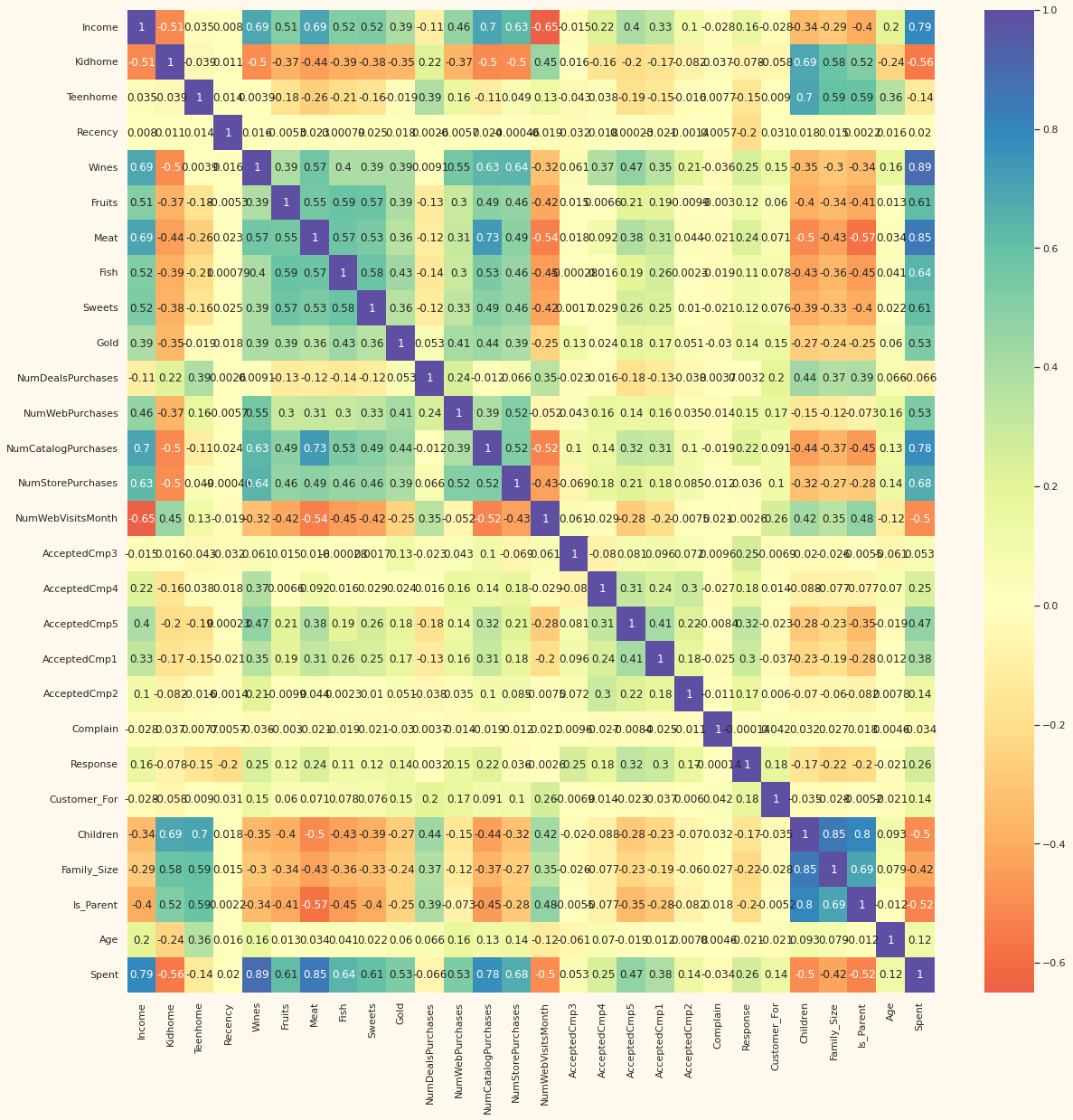
# correlation matrix 히트맵으로 표현하기
corrmat= df.corr()
plt.figure(figsize=(20,20))  
sns.heatmap(corrmat, annot=True, cmap="Spectral", center=0)

👣 데이터 전처리하기: Preprocessing

카테고리 형 데이터를 숫자형으로 바꾸기
피쳐 간 규모를 맞추기 위해 Scaling 하기
모델에 넣을 피쳐 - 차원 축소하기

카테고리 데이터 전처리하기

df.dtypes

=>

Education               object
Income                 float64
Kidhome                  int64
Teenhome                 int64
Recency                  int64
Wines                    int64
Fruits                   int64
Meat                     int64
Fish                     int64
Sweets                   int64
Gold                     int64
NumDealsPurchases        int64
NumWebPurchases          int64
NumCatalogPurchases      int64
NumStorePurchases        int64
NumWebVisitsMonth        int64
AcceptedCmp3             int64
AcceptedCmp4             int64
AcceptedCmp5             int64
AcceptedCmp1             int64
AcceptedCmp2             int64
Complain                 int64
Response                 int64
Customer_For             int64
Living_With             object
Children                 int64
Family_Size              int64
Is_Parent                int64
Age                      int64
Spent                    int64
dtype: object

# 데이터 중에서 object 의 데이터 형태를 가지고 있는 컬럼을 가져와라
s = (df.dtypes == 'object')
s[s.values == True].index
s[s].index 

=>

Index(['Education', 'Living_With'], dtype='object')

# 카테고리 형태의 데이터
s = (df.dtypes == 'object')
object_cols = list(s[s].index)

print("카테고리 데이터 종류:", object_cols)

=>

카테고리 데이터 종류: ['Education', 'Living_With']

# 카테고리 데이터에 라벨 인코더 사용하기
# 라벨 인코더란?
   # 카테고리형 데이터에 숫자를 매핑하여 바꿔준다. 
from sklearn.preprocessing import LabelEncoder

# Education 바꿔주기
LE=LabelEncoder()
df['Education']=df[['Education']].apply(LE.fit_transform)

df['Education'].head()

=>

0    0
1    0
2    0
3    0
4    1
Name: Education, dtype: int64

print(LE.classes_)
print(LE.inverse_transform([1, 2, 2]))

=>

['Graduate' 'Postgraduate' 'Undergraduate']
['Postgraduate' 'Undergraduate' 'Undergraduate']

# Living_With 카테고리 -> 숫자로 바꿔주기
df['Living_With']=df[['Living_With']].apply(LE.fit_transform)
df['Living_With'].head()

=>

0    0
1    0
2    1
3    1
4    1
Name: Living_With, dtype: int64

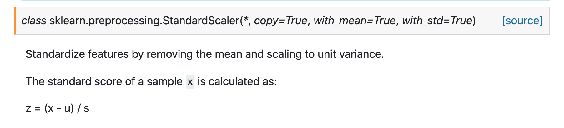
피쳐 간 규모를 맞추기 위해 Scaling 하기

from sklearn.preprocessing import StandardScaler

ds = df.copy()

# 나중에 클러스터 별 캠페인 반응률을 살펴보기 위해 사용
# 클러스터를 구성하기 위한 피쳐에서는 제거한다.
cols_del = ['AcceptedCmp3', 'AcceptedCmp4', 'AcceptedCmp5', 'AcceptedCmp1','AcceptedCmp2', 'Complain', 'Response']
ds = ds.drop(cols_del, axis=1)

ds.head()

	Education	Income	Kidhome	Teenhome	Recency	Wines	Fruits	Meat	Fish	Sweets	...	NumCatalogPurchases	NumStorePurchases	NumWebVisitsMonth	Customer_For	Living_With	Children	Family_Size	Is_Parent	Age	Spent
0	0	58138.0	0	0	58	635	88	546	172	88	...	10	4	7	83894400000000000	0	0	1	0	64	1617
1	0	46344.0	1	1	38	11	1	6	2	1	...	1	2	5	10800000000000000	0	2	3	1	67	27
2	0	71613.0	0	0	26	426	49	127	111	21	...	2	10	4	40780800000000000	1	0	2	0	56	776
3	0	26646.0	1	0	26	11	4	20	10	3	...	0	4	6	5616000000000000	1	1	3	1	37	53
4	1	58293.0	1	0	94	173	43	118	46	27	...	3	6	5	27734400000000000	1	1	3	1	40	422

#Scaling
scaler = StandardScaler()
scaler.fit(ds) # mean, variance 계산

# 적용
scaled_ds = pd.DataFrame(scaler.transform(ds), columns= ds.columns )
print("All features are now scaled")

=>

All features are now scaled

#Scaled data to be used for reducing the dimensionality
print("Dataframe to be used for further modelling:")
scaled_ds.head()

	Education	Income	Kidhome	Teenhome	Recency	Wines	Fruits	Meat	Fish	Sweets	...	NumCatalogPurchases	NumStorePurchases	NumWebVisitsMonth	Customer_For	Living_With	Children	Family_Size	Is_Parent	Age	Spent
0	-0.893586	0.287105	-0.822754	-0.929699	0.310353	0.977660	1.552041	1.690293	2.453472	1.483713	...	2.503607	-0.555814	0.692181	1.973583	-1.349603	-1.264598	-1.758359	-1.581139	1.018352	1.676245
1	-0.893586	-0.260882	1.040021	0.908097	-0.380813	-0.872618	-0.637461	-0.718230	-0.651004	-0.634019	...	-0.571340	-1.171160	-0.132545	-1.665144	-1.349603	1.404572	0.449070	0.632456	1.274785	-0.963297
2	-0.893586	0.913196	-0.822754	-0.929699	-0.795514	0.357935	0.570540	-0.178542	1.339513	-0.147184	...	-0.229679	1.290224	-0.544908	-0.172664	0.740959	-1.264598	-0.654644	-1.581139	0.334530	0.280110
3	-0.893586	-1.176114	1.040021	-0.929699	-0.795514	-0.872618	-0.561961	-0.655787	-0.504911	-0.585335	...	-0.913000	-0.555814	0.279818	-1.923210	0.740959	0.069987	0.449070	0.632456	-1.289547	-0.920135
4	0.571657	0.294307	1.040021	-0.929699	1.554453	-0.392257	0.419540	-0.218684	0.152508	-0.001133	...	0.111982	0.059532	-0.132545	-0.822130	0.740959	0.069987	0.449070	0.632456	-1.033114	-0.307562

여기까지 카테고리 데이터를 LabelEncoder 를 통해 숫자형으로 변환
Scaler 를 사용하여 데이터를 정규화

💡 Dimension Reduction

앞의 상관계수 행렬에서 봤듯이, 서로 관련있는 피쳐들이 많음.
변수가 너무 많으면, 모델링이 적절하게 되지 않을 수 있음.

-> 우리 데이터에 상관성이 많고, 피쳐가 너무 많은데 클러스터를 수행하려다 보니 PCA(차원 축소 기법)을 사용해서 차원을 축소 시켜 보자.

# PCA 로 3차원으로 데이터를 줄인다.
# sklearn 에서 PCA 모듈을 불러온다.
from sklearn.decomposition import PCA

pca = PCA(n_components=3)
pca.fit(scaled_ds)
PCA_ds = pd.DataFrame(pca.transform(scaled_ds), columns=(["col1","col2", "col3"]))

PCA_ds.describe().T

	count	mean	std	min	25%	50%	75%	max
col1	2212.0	-2.569775e-17	2.878377	-5.969394	-2.538494	-0.780421	2.383290	7.444305
col2	2212.0	-8.994212e-17	1.706839	-4.312106	-1.328321	-0.158197	1.242240	6.142664
col3	2212.0	7.388103e-17	1.221956	-3.530975	-0.828811	-0.021838	0.800092	6.615874

PCA_ds.head()

	col1	col2	col3
0	4.994347	-0.151233	2.647706
1	-2.884455	-0.006707	-1.863811
2	2.617864	-0.720806	-0.254408
3	-2.676036	-1.541954	-0.922951
4	-0.649591	0.209833	-0.021460

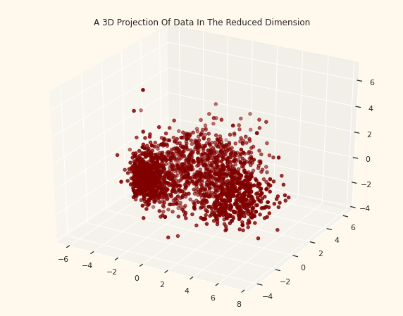
#A 3D Projection Of Data In The Reduced Dimension
x =PCA_ds["col1"]
y =PCA_ds["col2"]
z =PCA_ds["col3"]

#3D 플랏 그리기
# https://www.python-graph-gallery.com/370-3d-scatterplot
fig = plt.figure(figsize=(10,8))
ax = fig.add_subplot(111, projection="3d")
ax.scatter(x,y,z, c="maroon", marker="o" )
ax.set_title("A 3D Projection Of Data In The Reduced Dimension")
plt.show()

👣 유저 세그먼트 나누기: Clustering

💡 Elbow Method

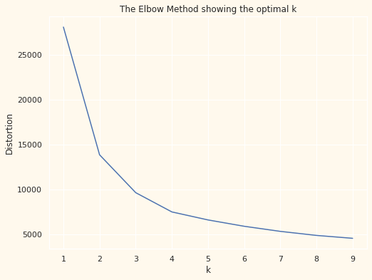
데이터를 몇 개로 나눠야 할까?

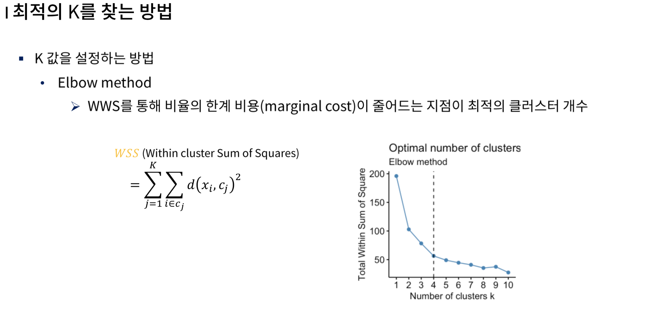
Elbow Method
WSS(군집 내 분산)은 작을 수록 군집의 중심에 많이 모여있는 것이므로 WSS(군집 내 분산)이 작을 수록 좋다.
하지만 클러스터를 늘려서 더 이상 작아지지 않는 한계점이 있다면 더 이상 클러스터 수를 증가시키지 않아도 좋다.

# 이미지 출처: https://heung-bae-lee.github.io/2020/05/30/machine_learning_19/

``py from sklearn.cluster import KMeans

```py
# Quick examination of elbow method to find numbers of clusters to make.
print('Elbow Method to determine the number of clusters to be formed:')

distortions = []

# 클러스터 개수 1 ~ 10 까지 늘려보면서
# 클러스터 내 거리합을 저장한다.
K = range(1,10)
for k in K:
    kmeanModel = KMeans(n_clusters=k)
    kmeanModel.fit(PCA_ds)
    distortions.append(kmeanModel.inertia_) # within-cluster sum-of-squares criterion

distortions

=>

[28060.968908252147,
123695080303,
179269985394,
577127923258,
895912178157,
488242066771,
942980809662,
552990155307,
679730812983]

plt.figure(figsize=(8,6))
plt.plot(K, distortions)
plt.xlabel('k')
plt.ylabel('Distortion')
plt.title('The Elbow Method showing the optimal k')
plt.show()

클러스터링을 해보자!

여기서는 Hierarchical Clustering 을 먼저 적용해 보았다.

from sklearn.cluster import AgglomerativeClustering


# 유사도 기준: affinity = euclidean
AC = AgglomerativeClustering(n_clusters=4)

# fit model and predict clusters
yhat_AC = AC.fit_predict(PCA_ds)
PCA_ds["Clusters"] = yhat_AC

# 기존 데이터에도 넣는다.
df["Clusters"]= yhat_AC

# Plotting the clusters
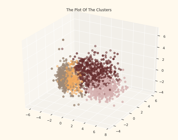
fig = plt.figure(figsize=(10,8))
ax = plt.subplot(111, projection='3d', label="bla")
ax.scatter(x, y, z, s=40, c=PCA_ds["Clusters"], marker='o', cmap = cmap )
ax.set_title("The Plot Of The Clusters")
plt.show()

👣 모델 평가하기: Evaluation

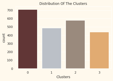
EDA 를 통해 만들어진 클러스터와 그 특성 파악하기 그룹이 골고루 분포되어 있을까?

# Plotting countplot of clusters
pal = ["#682F2F","#B9C0C9", "#9F8A78","#F3AB60"]
pl = sns.countplot(x=df["Clusters"], palette=pal)
pl.set_title("Distribution Of The Clusters")
plt.show()

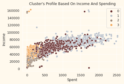
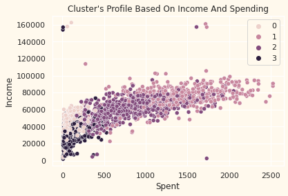
클러스터 별 구매금액과 연간 수입을 알아보자

pl = sns.scatterplot(data = df,x=df["Spent"], y=df["Income"],hue=df["Clusters"], palette= pal)
pl.set_title("Cluster's Profile Based On Income And Spending")
plt.legend()
plt.show()


# group 3: high spending & low income (3)
# group 2: low spending & low income (2)
# group 0: high spending & average income (0)
# group 1: high spending & high income (1)

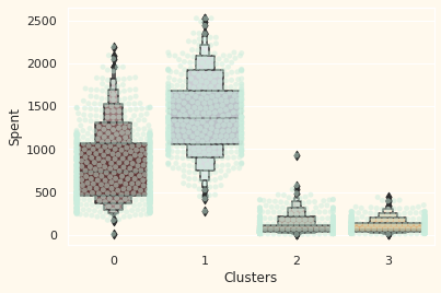
구매를 많이하는 고객층은?

plt.figure()
pl=sns.swarmplot(x=df["Clusters"], y=df["Spent"], color= "#CBEDDD", alpha=0.5 )
pl=sns.boxenplot(x=df["Clusters"], y=df["Spent"], palette=pal)

어떤 클러스터에서 캠페인 반응이 높을까?

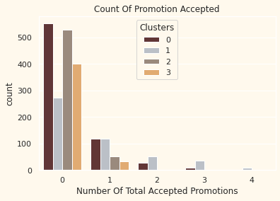
# Creating a feature to get a sum of accepted promotions 
df["Total_Promos"] = df["AcceptedCmp1"]+ df["AcceptedCmp2"]+ df["AcceptedCmp3"]+ df["AcceptedCmp4"]+ df["AcceptedCmp5"]

# Plotting count of total campaign accepted.
plt.figure()
pl = sns.countplot(x=df["Total_Promos"],hue=df["Clusters"], palette= pal)
pl.set_title("Count Of Promotion Accepted")
pl.set_xlabel("Number Of Total Accepted Promotions")
plt.show()

# 대부분 반응을 하지 않았다. 프로모션이 더 잘 디자인 될 필요가 있다.

할인에 잘 반응한 그룹은?

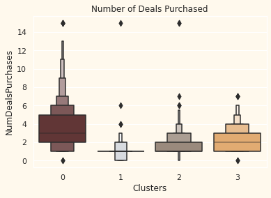
# Plotting the number of deals purchased
plt.figure()
pl=sns.boxenplot(y=df["NumDealsPurchases"],x=df["Clusters"], palette= pal)
pl.set_title("Number of Deals Purchased")
plt.show()

가족 구성원과 나이대는 어떻게 될까?

Personal = [ "Income","Kidhome","Teenhome","Customer_For", "Age", "Children", "Family_Size", "Is_Parent", "Education","Living_With"]

for i in Personal:
    plt.figure()
    sns.boxplot(y=df[i], x=df["Clusters"], palette=pal)
    plt.show()

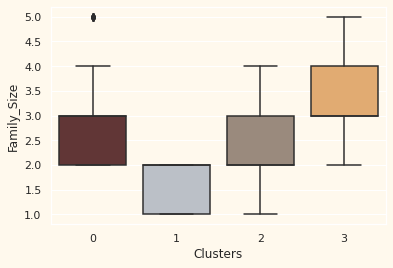
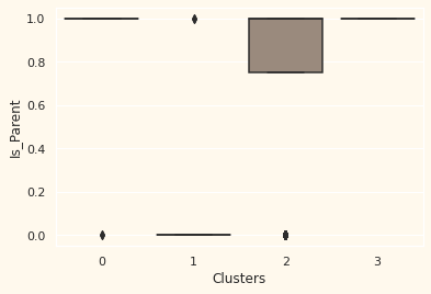
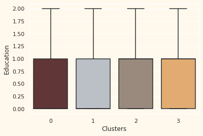
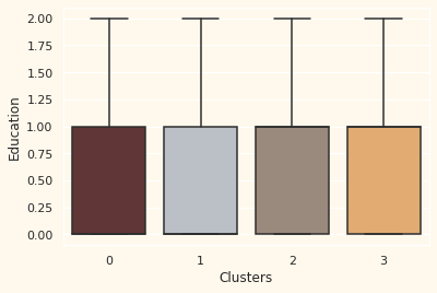
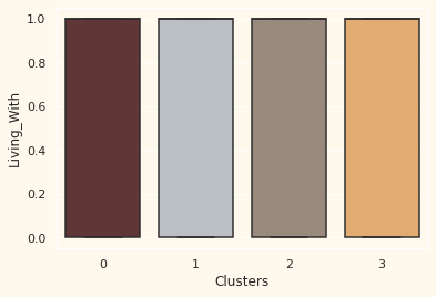
부모이며, 가족 구성원이 2 -4, 한부모 가정, 10대, 비교적 나이가 있음
부모가 아니며, 많아도 2명정도의 가족 구성원, 전 연령에 골고루 있음, 연간 수입이 높음
대부분 부모이며, 최대 4명의 가족 구성원, 10대가 아닌 1명의 어린 아이를 두고 있음, 상대적으로 어림
부모이며, 최대 5명까지의 가족 구성원, 상대적으로 나이가 있고, 수입이 낮음

👣 다양한 클러스터링 모델 사용해보기

💡Density Based Clustering

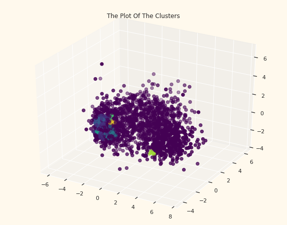
from sklearn.cluster import DBSCAN
# Initiating the DBSCAN Clustering model 
DP = DBSCAN(eps=0.30, min_samples=9)

# fit model and predict clusters
DP_df = DP.fit_predict(PCA_ds)
PCA_ds["DBSCAN_Clusters"] = DP_df

# Adding the Clusters feature to the orignal dataframe.
df["DBSCAN_Clusters"]= DP_df

# Plotting the clusters
fig = plt.figure(figsize=(10,8))
ax = plt.subplot(111, projection='3d', label="bla")
ax.scatter(x, y, z, s=40, c=PCA_ds["DBSCAN_Clusters"], marker='o', cmap = 'viridis' )
ax.set_title("The Plot Of The Clusters")
plt.show()

# Plotting countplot of clusters
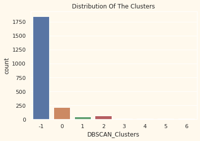
pl = sns.countplot(x=df["DBSCAN_Clusters"])
pl.set_title("Distribution Of The Clusters")
plt.show()

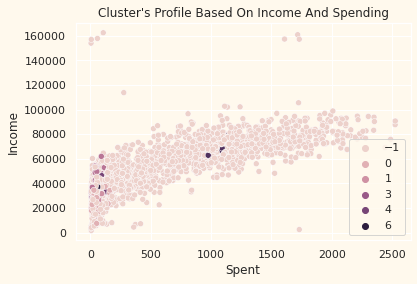
pl = sns.scatterplot(data = df,x=df["Spent"], y=df["Income"],hue=df["DBSCAN_Clusters"])
pl.set_title("Cluster's Profile Based On Income And Spending")
plt.legend()
plt.show()

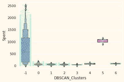
plt.figure()
pl=sns.swarmplot(x=df["DBSCAN_Clusters"], y=df["Spent"], color= "#CBEDDD", alpha=0.5 )
pl=sns.boxenplot(x=df["DBSCAN_Clusters"], y=df["Spent"])
plt.show()

💡Partition Based Clustering

Kmeans = KMeans(n_clusters=4)
# fit model and predict clusters
Kmeans_df = Kmeans.fit_predict(PCA_ds)
PCA_ds["Kmeans_Clusters"] = Kmeans_df
#Adding the Clusters feature to the orignal dataframe.
df["Kmeans_Clusters"]= Kmeans_df

#Plotting countplot of clusters
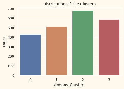
pl = sns.countplot(x=df["Kmeans_Clusters"])
pl.set_title("Distribution Of The Clusters")
plt.show()

pl = sns.scatterplot(data = df,x=df["Spent"], y=df["Income"],hue=df["Kmeans_Clusters"])
pl.set_title("Cluster's Profile Based On Income And Spending")
plt.legend()
plt.show()

💡 Silhouette Coefficient

from sklearn.metrics import silhouette_samples

# Hierachical
sample_silhouette_values = silhouette_samples(PCA_ds, PCA_ds["Clusters"])
print("Hierachical",sample_silhouette_values.mean())

# Density - DBSCAN
sample_silhouette_values = silhouette_samples(PCA_ds, PCA_ds["DBSCAN_Clusters"])
print("Density",sample_silhouette_values.mean())


# Kmeans
sample_silhouette_values = silhouette_samples(PCA_ds, PCA_ds["Kmeans_Clusters"])
print("Kmeans",sample_silhouette_values.mean())

=>

Hierachical 0.45273806967143565
Density 0.05700586237988258
Kmeans 0.46554372154673307

Twitter Facebook LinkedIn

Project 9 - 유저 군집 분석

클러스터링, 군집화

언제 사용할까?

유사한 뉴스 그룹 : 문서 군집화

가까운 위치 좌표끼리 묶기

유사한 유저군 나누기 : 마켓 세분화

종류

Partition-based Clustering

Hierarchical based Clustering

Centroid Distance

Median Distance

Density based Clustering

DBSCAN clustering

정답이 없는 클러스터링, 어떻게 평가할까?

Silhouette Coefficient: 실루엣 계수

다양한 클러스터링 방법을 통해 유저 세그먼트를 나눠보자

라이브러리 불러오기

👣 데이터 살펴보기

데이터 컬럼 종류

People (사람)

Products (상품)

Promotion (프로모션)

Place (구매 장소)

👣 데이터 정제하기: Cleaning

💡 Correlation Coefficients

👣 데이터 전처리하기: Preprocessing

💡 Dimension Reduction

👣 유저 세그먼트 나누기: Clustering

💡 Elbow Method

👣 모델 평가하기: Evaluation

👣 다양한 클러스터링 모델 사용해보기

💡Density Based Clustering

💡Partition Based Clustering

💡 Silhouette Coefficient

공유하기

참고

Project 3 - Web Parsing

Project 4 - 시카고 맛집 데이터 분석

Project 8 - 인구 소멸 위기 지역 데이터 분석

Project 5 - 네이버 영화 평점 사이트 분석

클러스터링, 군집화

언제 사용할까?

유사한 뉴스 그룹 : 문서 군집화

가까운 위치 좌표끼리 묶기

유사한 유저군 나누기 : 마켓 세분화

SNS 관심사 기반, 자율 주행 이미지 인식 클러스터링

종류

Partition-based Clustering

Hierarchical based Clustering

Centroid Distance

Median Distance

Density based Clustering

DBSCAN clustering

정답이 없는 클러스터링, 어떻게 평가할까?

Silhouette Coefficient: 실루엣 계수

다양한 클러스터링 방법을 통해 유저 세그먼트를 나눠보자

라이브러리 불러오기

👣 데이터 살펴보기

데이터 컬럼 종류

People (사람)

Products (상품)

Promotion (프로모션)

Place (구매 장소)

👣 데이터 정제하기: Cleaning

💡 Correlation Coefficients

👣 데이터 전처리하기: Preprocessing

💡 Dimension Reduction

👣 유저 세그먼트 나누기: Clustering

💡 Elbow Method

👣 모델 평가하기: Evaluation

👣 다양한 클러스터링 모델 사용해보기

💡Density Based Clustering

💡Partition Based Clustering

💡 Silhouette Coefficient

공유하기

참고

Project 3 - Web Parsing

Project 4 - 시카고 맛집 데이터 분석

Project 8 - 인구 소멸 위기 지역 데이터 분석

Project 5 - 네이버 영화 평점 사이트 분석