Project 2 - 서울시 범죄 현황 데이터 분석 (3)

August 25, 2024 8 분 소요

범죄 데이터 정렬을 위한 데이터 정리

crime_anal_gu.head()

	강간	강도	살인	절도	폭력	강간검거율	강도검거율	살인검거율	절도검거율	폭력검거율
구별
강남구	516.0	39.0	5.0	3587.0	4002.0	80.038760	100.000000	100.000000	53.470867	88.130935
강동구	160.0	14.0	4.0	1754.0	2530.0	95.000000	92.857143	100.000000	51.425314	86.996047
강북구	217.0	5.0	7.0	1222.0	2778.0	73.271889	80.000000	85.714286	54.991817	89.344852
관악구	322.0	12.0	6.0	2103.0	3235.0	81.987578	83.333333	100.000000	44.555397	83.678516
광진구	279.0	11.0	4.0	2636.0	2392.0	83.870968	54.545455	100.000000	40.098634	84.071906

정규화

#최대값 1, 최소값 0
crime_anal_gu["강도"] / crime_anal_gu["강도"].max()

구별
강남구     1.000000
강동구     0.358974
강북구     0.128205
관악구     0.307692
광진구     0.282051
구로구     0.256410
금천구     0.179487
노원구     0.153846
도봉구     0.128205
동대문구    0.256410
동작구     0.179487
마포구     0.102564
서대문구    0.128205
서초구     0.333333
성동구     0.076923
성북구     0.205128
송파구     0.384615
양천구     0.435897
영등포구    0.487179
용산구     0.230769
은평구     0.230769
종로구     0.307692
중구      0.205128
중랑구     0.358974
Name: 강도, dtype: float64

col = ["살인", "강도", "강간", "절도", "폭력"]
crime_anal_norm = crime_anal_gu[col] / crime_anal_gu[col].max()
crime_anal_norm.head()

	살인	강도	강간	절도	폭력
구별
강남구	0.357143	1.000000	1.000000	0.977118	0.733773
강동구	0.285714	0.358974	0.310078	0.477799	0.463880
강북구	0.500000	0.128205	0.420543	0.332879	0.509351
관악구	0.428571	0.307692	0.624031	0.572868	0.593143
광진구	0.285714	0.282051	0.540698	0.718060	0.438577

검거율 추가

col2 = ["강간검거율", "강도검거율", "살인검거율", "절도검거율", "폭력검거율"]
crime_anal_norm[col2] = crime_anal_gu[col2]
crime_anal_norm.head()

	살인	강도	강간	절도	폭력	강간검거율	강도검거율	살인검거율	절도검거율	폭력검거율
구별
강남구	0.357143	1.000000	1.000000	0.977118	0.733773	80.038760	100.000000	100.000000	53.470867	88.130935
강동구	0.285714	0.358974	0.310078	0.477799	0.463880	95.000000	92.857143	100.000000	51.425314	86.996047
강북구	0.500000	0.128205	0.420543	0.332879	0.509351	73.271889	80.000000	85.714286	54.991817	89.344852
관악구	0.428571	0.307692	0.624031	0.572868	0.593143	81.987578	83.333333	100.000000	44.555397	83.678516
광진구	0.285714	0.282051	0.540698	0.718060	0.438577	83.870968	54.545455	100.000000	40.098634	84.071906

구별 CCTV자료에서 인구수, CCTV 수 추가

result_CCTV = pd.read_csv("../data/01. CCTV_result.csv", index_col="구별", encoding="utf-8")
result_CCTV.head()

	소계	최근증가율	인구수	한국인	외국인	고령자	외국인비율	고령자비율	CCTV비율	오차
구별
강남구	3238	150.619195	561052	556164	4888	65060	0.871220	11.596073	0.577130	1549.200326
강동구	1010	166.490765	440359	436223	4136	56161	0.939234	12.753458	0.229358	-544.642322
강북구	831	125.203252	328002	324479	3523	56530	1.074079	17.234651	0.253352	-598.750923
강서구	911	134.793814	608255	601691	6564	76032	1.079153	12.500021	0.149773	-830.268578
관악구	2109	149.290780	520929	503297	17632	70046	3.384722	13.446362	0.404854	464.799395

crime_anal_norm[["인구수", "CCTV"]] = result_CCTV[["인구수", "소계"]]
crime_anal_norm.head()

	살인	강도	강간	절도	폭력	강간검거율	강도검거율	살인검거율	절도검거율	폭력검거율	인구수	CCTV
구별
강남구	0.357143	1.000000	1.000000	0.977118	0.733773	80.038760	100.000000	100.000000	53.470867	88.130935	561052	3238
강동구	0.285714	0.358974	0.310078	0.477799	0.463880	95.000000	92.857143	100.000000	51.425314	86.996047	440359	1010
강북구	0.500000	0.128205	0.420543	0.332879	0.509351	73.271889	80.000000	85.714286	54.991817	89.344852	328002	831
관악구	0.428571	0.307692	0.624031	0.572868	0.593143	81.987578	83.333333	100.000000	44.555397	83.678516	520929	2109
광진구	0.285714	0.282051	0.540698	0.718060	0.438577	83.870968	54.545455	100.000000	40.098634	84.071906	372298	878

정규화된 범죄발생 건수 전체 평균을 구해서 범죄 컬럼 대표값으로 사용

col = ["강간", "강도", "살인", "절도", "폭력"]
crime_anal_norm["범죄"] = np.mean(crime_anal_norm[col], axis=1) #행렬의 평균
crime_anal_norm.head()

Out[112]:

	살인	강도	강간	절도	폭력	강간검거율	강도검거율	살인검거율	절도검거율	폭력검거율	인구수	CCTV	범죄
구별
강남구	0.357143	1.000000	1.000000	0.977118	0.733773	80.038760	100.000000	100.000000	53.470867	88.130935	561052	3238	0.813607
강동구	0.285714	0.358974	0.310078	0.477799	0.463880	95.000000	92.857143	100.000000	51.425314	86.996047	440359	1010	0.379289
강북구	0.500000	0.128205	0.420543	0.332879	0.509351	73.271889	80.000000	85.714286	54.991817	89.344852	328002	831	0.378196
관악구	0.428571	0.307692	0.624031	0.572868	0.593143	81.987578	83.333333	100.000000	44.555397	83.678516	520929	2109	0.505261
광진구	0.285714	0.282051	0.540698	0.718060	0.438577	83.870968	54.545455	100.000000	40.098634	84.071906	372298	878	0.453020

np.mean()

np.array(
    [[0.357143, 1.000000, 1.000000, 0.977118, 0.733773],
    [0.285714, 0.358974, 0.310078, 0.477799, 0.463880]]
)

=>

array([[0.357143, 1.      , 1.      , 0.977118, 0.733773],
       [0.285714, 0.358974, 0.310078, 0.477799, 0.46388 ]])

------------------------------------------------------------
       
np.mean(np.array(
    [[0.357143, 1.000000, 1.000000, 0.977118, 0.733773],
    [0.285714, 0.358974, 0.310078, 0.477799, 0.463880]]
), axis=1) # axis=1 : 행 기준, axis=0 : 열 기준

=>

array([0.8136068, 0.379289 ])

검거율의 평균을 검거 컬럼의 대표값으로 사용

col = ["강간검거율", "강도검거율", "살인검거율", "절도검거율", "폭력검거율"]
crime_anal_norm["검거"] = np.mean(crime_anal_norm[col], axis=1) # axis=1 : 행 기준
crime_anal_norm.head()

	살인	강도	강간	절도	폭력	강간검거율	강도검거율	살인검거율	절도검거율	폭력검거율	인구수	CCTV	범죄	검거
구별
강남구	0.357143	1.000000	1.000000	0.977118	0.733773	80.038760	100.000000	100.000000	53.470867	88.130935	561052	3238	0.813607	84.328112
강동구	0.285714	0.358974	0.310078	0.477799	0.463880	95.000000	92.857143	100.000000	51.425314	86.996047	440359	1010	0.379289	85.255701
강북구	0.500000	0.128205	0.420543	0.332879	0.509351	73.271889	80.000000	85.714286	54.991817	89.344852	328002	831	0.378196	76.664569
관악구	0.428571	0.307692	0.624031	0.572868	0.593143	81.987578	83.333333	100.000000	44.555397	83.678516	520929	2109	0.505261	78.710965
광진구	0.285714	0.282051	0.540698	0.718060	0.438577	83.870968	54.545455	100.000000	40.098634	84.071906	372298	878	0.453020	72.517393

최종 데이터 프레임

crime_anal_norm

	살인	강도	강간	절도	폭력	강간검거율	강도검거율	살인검거율	절도검거율	폭력검거율	인구수	CCTV	범죄	검거
구별
강남구	0.357143	1.000000	1.000000	0.977118	0.733773	80.038760	100.000000	100.000000	53.470867	88.130935	561052	3238	0.813607	84.328112
강동구	0.285714	0.358974	0.310078	0.477799	0.463880	95.000000	92.857143	100.000000	51.425314	86.996047	440359	1010	0.379289	85.255701
강북구	0.500000	0.128205	0.420543	0.332879	0.509351	73.271889	80.000000	85.714286	54.991817	89.344852	328002	831	0.378196	76.664569
관악구	0.428571	0.307692	0.624031	0.572868	0.593143	81.987578	83.333333	100.000000	44.555397	83.678516	520929	2109	0.505261	78.710965
광진구	0.285714	0.282051	0.540698	0.718060	0.438577	83.870968	54.545455	100.000000	40.098634	84.071906	372298	878	0.453020	72.517393
구로구	0.642857	0.256410	0.529070	0.520294	0.580125	66.300366	100.000000	100.000000	45.078534	84.702908	441559	1884	0.505751	79.216362
금천구	0.428571	0.179487	0.339147	0.344320	0.402090	81.714286	100.000000	100.000000	51.740506	88.736890	253491	1348	0.338723	84.438336
노원구	0.357143	0.153846	0.308140	0.505857	0.461313	89.308176	100.000000	100.000000	39.849219	84.419714	558075	1566	0.357260	82.715422
도봉구	0.214286	0.128205	0.238372	0.235903	0.264210	98.373984	100.000000	100.000000	56.812933	90.839695	346234	825	0.216195	89.205322
동대문구	0.357143	0.256410	0.368217	0.528466	0.484415	83.157895	100.000000	100.000000	55.206186	89.969720	366011	1870	0.398930	85.666760
동작구	0.571429	0.179487	0.629845	0.333969	0.304547	45.846154	100.000000	75.000000	45.187602	86.935581	408493	1302	0.403855	70.593867
마포구	0.285714	0.102564	0.773256	0.688368	0.538871	80.200501	100.000000	100.000000	37.198259	85.062947	385783	980	0.477755	80.492341
서대문구	0.428571	0.128205	0.339147	0.409425	0.362303	84.000000	80.000000	100.000000	50.033267	83.198381	325028	1254	0.333530	79.446329
서초구	0.357143	0.333333	0.829457	0.600654	0.428676	63.317757	76.923077	100.000000	50.204082	86.783576	445401	2297	0.509853	75.445698
성동구	0.285714	0.076923	0.201550	0.353037	0.296846	75.000000	100.000000	100.000000	69.135802	86.967264	312711	1327	0.242814	86.220613
성북구	0.285714	0.205128	0.298450	0.400436	0.386505	75.974026	100.000000	75.000000	49.319728	86.290323	455407	1651	0.315247	77.316815
송파구	0.642857	0.384615	0.453488	0.692727	0.603044	78.632479	80.000000	88.888889	41.211168	85.375494	671173	1081	0.555346	74.821606
양천구	1.000000	0.435897	0.786822	1.000000	1.000000	85.467980	100.000000	100.000000	49.713974	85.918592	475018	2482	0.844544	84.220109
영등포구	0.928571	0.487179	0.689922	0.637701	0.658783	63.202247	73.684211	100.000000	40.153780	83.690509	402024	1277	0.680431	72.146149
용산구	0.285714	0.230769	0.486434	0.405612	0.437110	85.258964	100.000000	100.000000	40.228341	84.228188	244444	2096	0.369128	81.943099
은평구	0.428571	0.230769	0.302326	0.453827	0.488449	91.025641	77.777778	100.000000	53.421369	86.636637	491202	2108	0.380788	81.772285
종로구	0.428571	0.307692	0.461240	0.528466	0.414925	74.369748	75.000000	33.333333	39.587629	87.361909	164257	1619	0.428179	61.930524
중구	0.214286	0.205128	0.383721	0.585671	0.407957	74.747475	87.500000	100.000000	42.511628	89.707865	134593	1023	0.359353	78.893394
중랑구	0.571429	0.358974	0.317829	0.460637	0.580125	91.463415	100.000000	87.500000	62.211709	85.714286	412780	916	0.457799	85.377882

Seaborn

import numpy as np
import pandas as pd
import matplotlib.pyplot as plt
import seaborn as sns
from matplotlib import rc

plt.rcParams["axes.unicode_minus"] = False
rc("font", family="malgun gothic")
%matplotlib inline # get_ipython().run_line_magic("matplotlib", "inline")

np.linspace(0, 14, 100) # 0부터 14까지 100개

=>

array([ 0.        ,  0.14141414,  0.28282828,  0.42424242,  0.56565657,
									.
                                    .
                                    .
       13.43434343, 13.57575758, 13.71717172, 13.85858586, 14.        ])

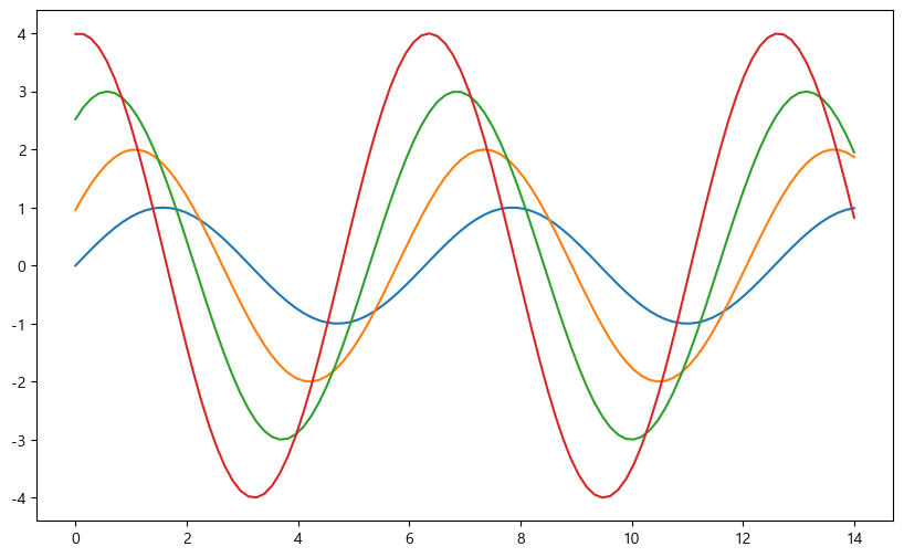
x = np.linspace(0, 14, 100)
y1 = np.sin(x)
y2 = 2 * np.sin(x + 0.5)
y3 = 3 * np.sin(x + 1.0)
y4 = 4 * np.sin(x + 1.5)

plt.figure(figsize=(10, 6))
plt.plot(x, y1, x, y2, x, y3, x, y4)
plt.show()

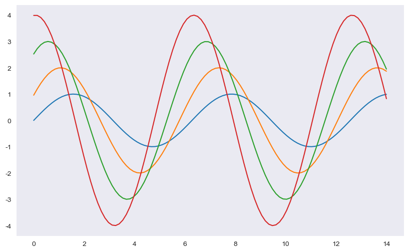
style : “white”, “whitegrid”, “dark”, “darkgrid”

sns.set_style("dark")
plt.figure(figsize=(10, 6))
plt.plot(x, y1, x, y2, x, y3, x, y4)
plt.show()

seaborn tips data

boxplot
swarmplot
lmplot

tips = sns.load_dataset("tips")
tips

	total_bill	tip	sex	smoker	day	time	size
0	16.99	1.01	Female	No	Sun	Dinner	2
1	10.34	1.66	Male	No	Sun	Dinner	3
2	21.01	3.50	Male	No	Sun	Dinner	3
3	23.68	3.31	Male	No	Sun	Dinner	2
4	24.59	3.61	Female	No	Sun	Dinner	4
...	...	...	...	...	...	...	...
239	29.03	5.92	Male	No	Sat	Dinner	3
240	27.18	2.00	Female	Yes	Sat	Dinner	2
241	22.67	2.00	Male	Yes	Sat	Dinner	2
242	17.82	1.75	Male	No	Sat	Dinner	2
243	18.78	3.00	Female	No	Thur	Dinner	2

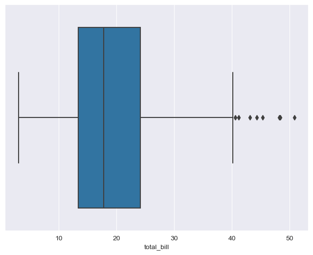
boxplot

plt.figure(figsize=(8, 6))
sns.boxplot(x=tips["total_bill"])
plt.show()

plt.figure(figsize=(8, 6))
sns.boxplot(x="day", y="total_bill", data=tips)
plt.show()

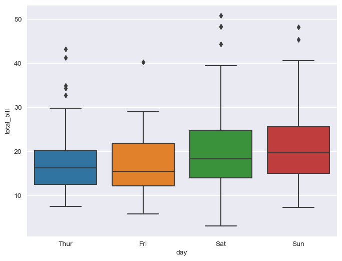
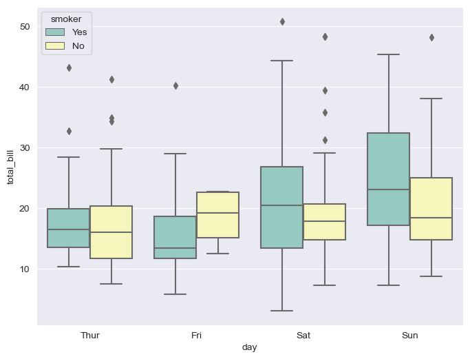
boxplot hue, palette option

# hue: 카테고리 데이터 표현

plt.figure(figsize=(8, 6))
sns.boxplot(x="day", y="total_bill", data=tips, hue="smoker", palette="Set3") # Set 1 ~ 3
plt.show()

swarmplot

color : 0~1 사이 -> 검은색부터 흰색 사이 값 조절

plt.figure(figsize=(8, 6))
sns.swarmplot(x="day", y="total_bill", data=tips, color="0")
plt.show()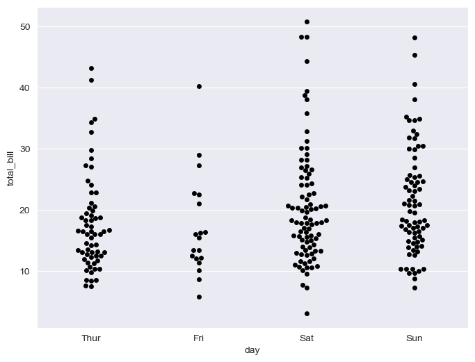

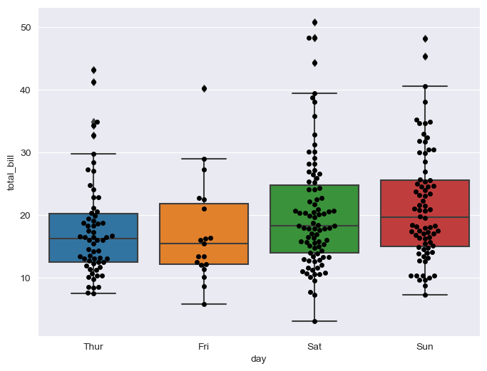
boxplot with swarmplot

plt.figure(figsize=(8, 6))
sns.boxplot(x="day", y="total_bill", data=tips)
sns.swarmplot(x="day", y="total_bill", data=tips, color="0")
plt.show()

lmplot

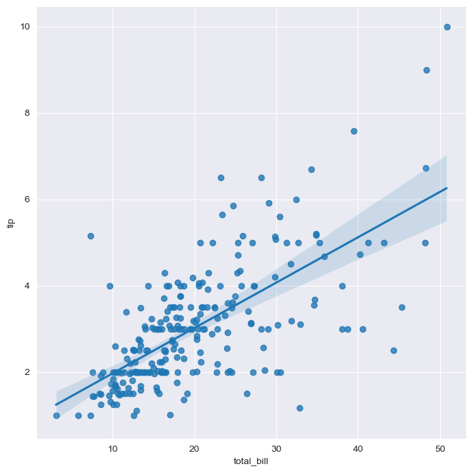
total_bill과 tip 사이 관계 파악

sns.set_style("darkgrid")
sns.lmplot(x="total_bill", y="tip", data=tips, height=7) # size => height
plt.show()

hue option

sns.set_style("darkgrid")
sns.lmplot(x="total_bill", y="tip", data=tips, height=7, hue="smoker")
plt.show()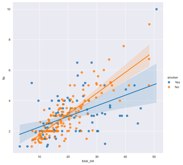

flights datas

heatmap

flights = sns.load_dataset("flights")
flights.head()

	year	month	passengers
0	1949	Jan	112
1	1949	Feb	118
2	1949	Mar	132
3	1949	Apr	129
4	1949	May	121

pivot(index, columns, values)

flights = flights.pivot(index="month", columns="year", values="passengers")
flights.head()

year	1949	1950	1951	1952	1953	1954	1955	1956	1957	1958	1959	1960
month
Jan	112	115	145	171	196	204	242	284	315	340	360	417
Feb	118	126	150	180	196	188	233	277	301	318	342	391
Mar	132	141	178	193	236	235	267	317	356	362	406	419
Apr	129	135	163	181	235	227	269	313	348	348	396	461
May	121	125	172	183	229	234	270	318	355	363	420	472

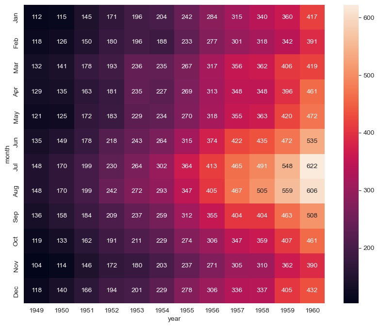
heatmap

plt.figure(figsize=(10, 8))
sns.heatmap(data=flights, annot=True, fmt="d") # annot=True : 데이터 값 표시, fmt="d" : 정수형 표현
plt.show()

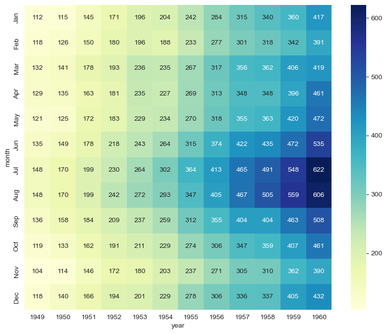
colormap

plt.figure(figsize=(10, 8))
sns.heatmap(flights, annot=True, fmt="d", cmap="YlGnBu")
plt.show()

iris data

pairplot

iris = sns.load_dataset("iris")
iris.tail()

	sepal_length	sepal_width	petal_length	petal_width	species
145	6.7	3.0	5.2	2.3	virginica
146	6.3	2.5	5.0	1.9	virginica
147	6.5	3.0	5.2	2.0	virginica
148	6.2	3.4	5.4	2.3	virginica
149	5.9	3.0	5.1	1.8	virginica

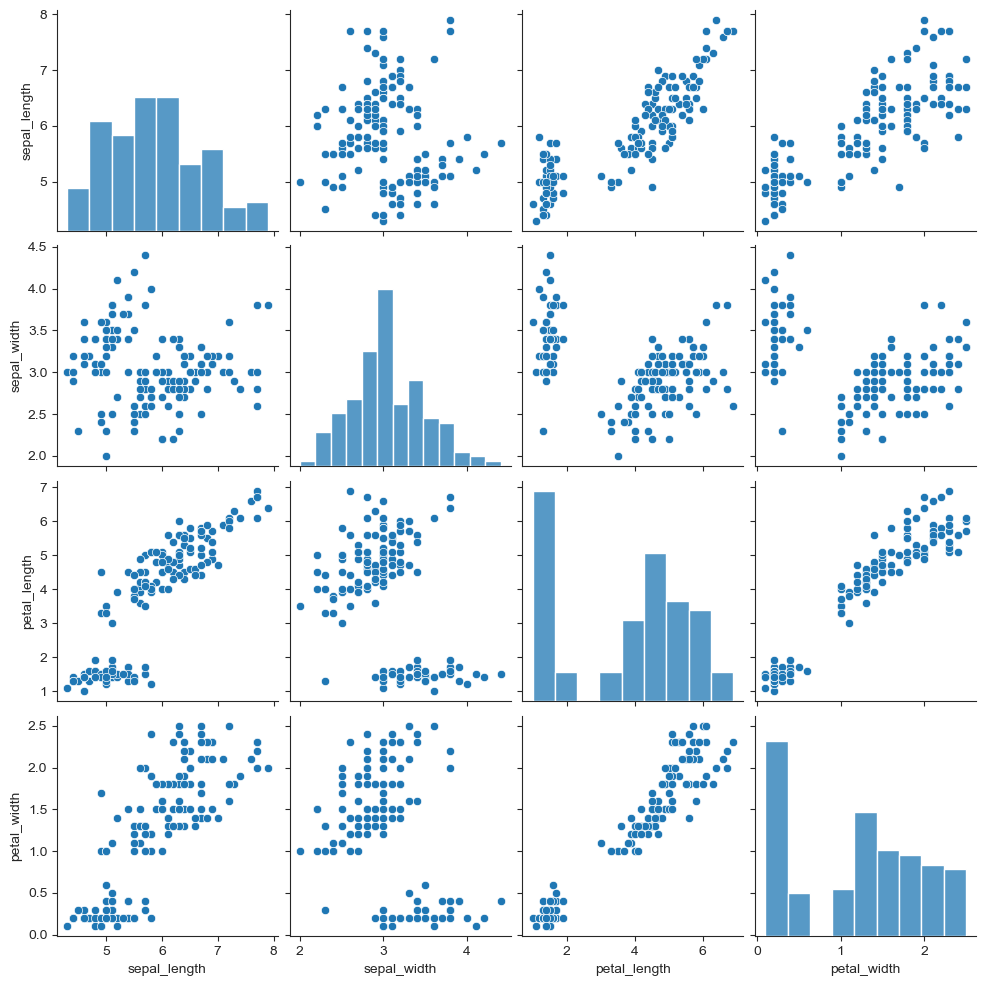
pairplot

sns.set_style("ticks")
sns.pairplot(iris)
plt.show()

hue option

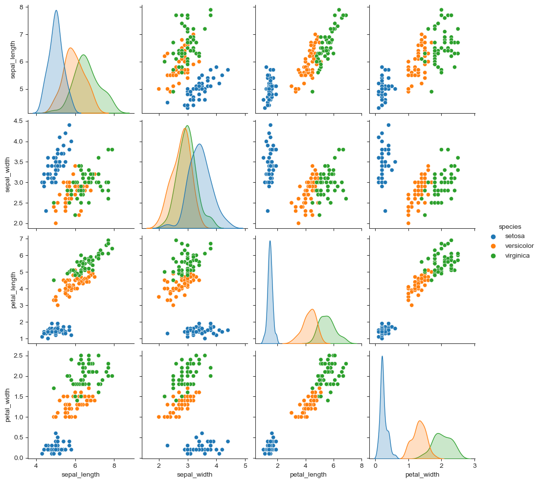
sns.pairplot(iris, hue="species")
plt.show()

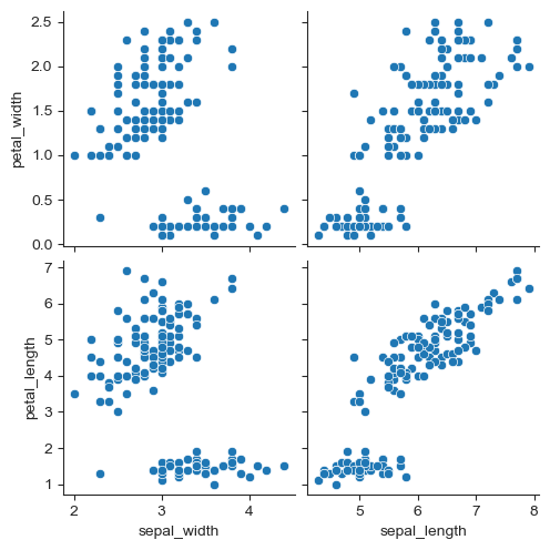
원하는 컬럼만 pairplot

sns.pairplot(iris, x_vars=["sepal_width", "sepal_length"], 
                   y_vars=["petal_width", "petal_length"])
plt.show()

anscombe data

lmplot

anscombe = sns.load_dataset("anscombe")
anscombe.tail()

	dataset	x	y
39	IV	8.0	5.25
40	IV	19.0	12.50
41	IV	8.0	5.56
42	IV	8.0	7.91
43	IV	8.0	6.89

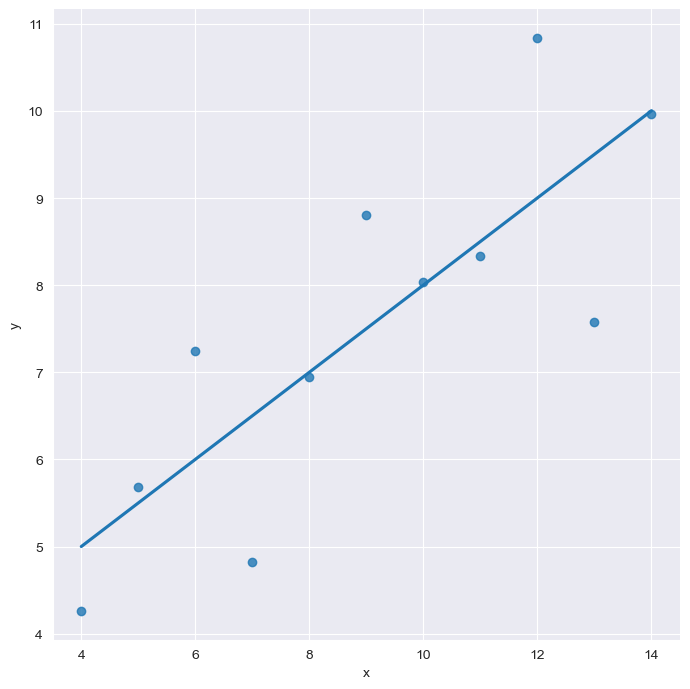
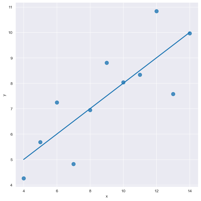
lmplot

sns.set_style("darkgrid")
sns.lmplot(x="x", y="y", data=anscombe.query("dataset == 'I'"), ci=None, height=7) # ci : 신뢰구간 선택
plt.show()

scatter 크기 조정

sns.set_style("darkgrid")
sns.lmplot(x="x", y="y", data=anscombe.query("dataset == 'I'"), ci=None, height=7, scatter_kws={"s":80}) # ci : 신뢰구간 선택
plt.show()

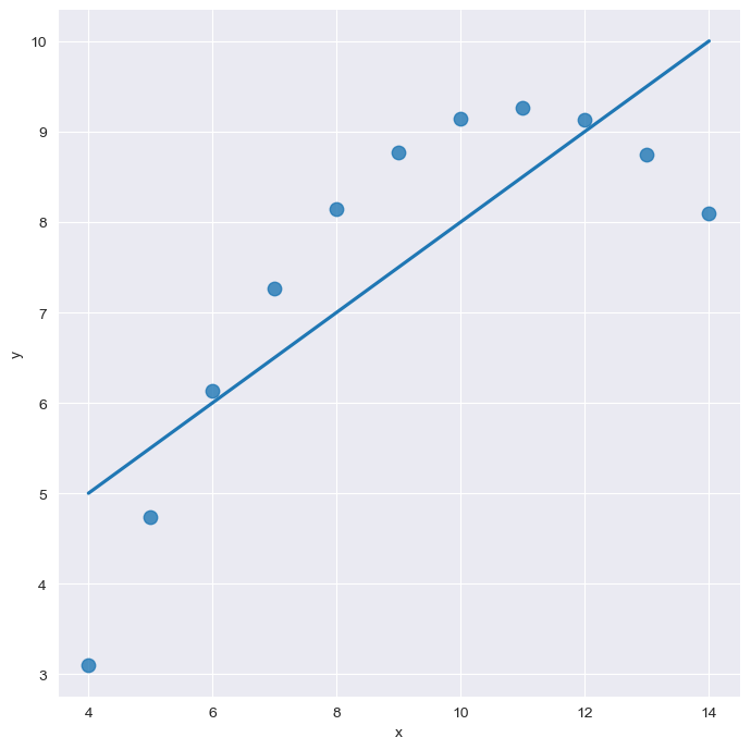
order option

sns.set_style("darkgrid")
sns.lmplot(
    x="x",
    y="y",
    data=anscombe.query("dataset == 'II'"),
    order=1,
    ci=None, height=7,
    scatter_kws={"s":80}) # ci : 신뢰구간 선택
plt.show()

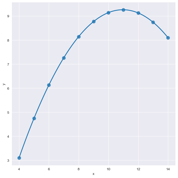
sns.set_style("darkgrid")
sns.lmplot(
    x="x",
    y="y",
    data=anscombe.query("dataset == 'II'"),
    order=2,
    ci=None, height=7,
    scatter_kws={"s":80}) # ci : 신뢰구간 선택
plt.show()

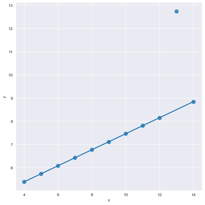
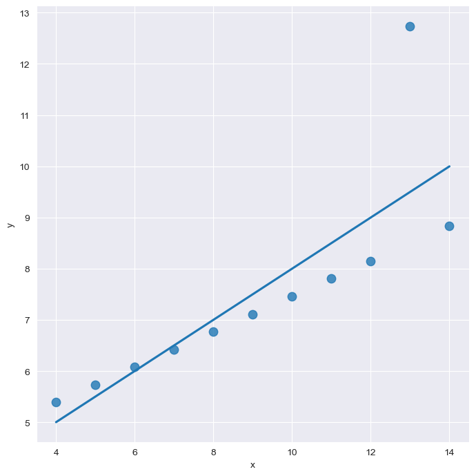
outliner

sns.set_style("darkgrid")
sns.lmplot(
    x="x",
    y="y",
    data=anscombe.query("dataset == 'III'"),
    ci=None, height=7,
    scatter_kws={"s" : 80}) # ci : 신뢰구간 선택
plt.show()

robust

sns.set_style("darkgrid")
sns.lmplot(
    x="x",
    y="y",
    data=anscombe.query("dataset == 'III'"),
    robust=True,
    ci=None,
    height=7,
    scatter_kws={"s" : 80}) # ci : 신뢰구간 선택
plt.show()

Twitter Facebook LinkedIn

Project 2 - 서울시 범죄 현황 데이터 분석 (3)

범죄 데이터 정렬을 위한 데이터 정리

정규화

검거율 추가

구별 CCTV자료에서 인구수, CCTV 수 추가

정규화된 범죄발생 건수 전체 평균을 구해서 범죄 컬럼 대표값으로 사용

np.mean()

검거율의 평균을 검거 컬럼의 대표값으로 사용

최종 데이터 프레임

Seaborn

style : “white”, “whitegrid”, “dark”, “darkgrid”

seaborn tips data

boxplot

boxplot hue, palette option

swarmplot

boxplot with swarmplot

lmplot

flights datas

pivot(index, columns, values)

heatmap

colormap

iris data

pairplot

원하는 컬럼만 pairplot

anscombe data

lmplot

scatter 크기 조정

order option

outliner

robust

공유하기

참고

Project 3 - Web Parsing

Project 4 - 시카고 맛집 데이터 분석

Project 8 - 인구 소멸 위기 지역 데이터 분석

Project 5 - 네이버 영화 평점 사이트 분석